![[DBPP]](pictures//asm_color_tiny.gif)


![[Search]](pictures//search_motif.gif)
Next: 2.7 Case Study: Floorplan Optimization
Up: 2 Designing Parallel Algorithms
Previous: 2.5 Mapping
In the next three sections, we develop parallel algorithms for
atmosphere modeling, VLSI design, and computational chemistry
problems. These case studies are intended to illustrate both the
design principles presented in the text and the
stepwise process by which realistic parallel algorithms are developed.
While the problems examined in these case studies are of considerable
interest in their own right, our interest here is in their
computational characteristics. The atmosphere modeling application
is an example of a problem amenable to parallelization by using
simple domain decomposition techniques. It is representative of a
wide range of scientific and engineering computations. The VLSI
design problem is an example of an irregular problem
requiring load-balancing techniques. It is representative of many
symbolic computing problems. Finally, the computational chemistry
application is an example of a problem requiring asynchronous access
to distributed data structures, a requirement that arises frequently
in both numerical and symbolic computing.
In each case study, we first briefly introduce the problem being
solved and then develop parallel algorithms. We restrict the problem
descriptions to essential computational issues and omit details that
would add to the length of the presentation without illustrating new
principles. In particular, we do not say much about why the
underlying scientific or engineering problem is formulated in the way
described, or about alternative problem formulations that might admit
to alternative parallelization strategies. The chapter notes provide
pointers to detailed treatments of these topics.
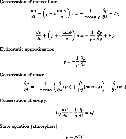
Figure 2.20: The basic predictive equations used in atmospheric
modeling, where  and
and  are latitude and longitude,
z
is height, u
and v
are horizontal components of
velocity, p
is pressure,
  is density, T
is
temperature, f
is Coriolis force, g
is gravity,
F
and Q
are external forcing terms,
  is specific
heat, and a
is the earth's radius.
An atmosphere model
is a computer program that simulates
atmospheric processes (wind, clouds, precipitation, etc.) that
influence weather or climate. It may be used to study the evolution
of tornadoes, to predict tomorrow's weather, or to study the impact on
climate of increased concentrations of atmospheric carbon dioxide.
Like many numerical models of physical processes, an atmosphere model
solves a set of partial differential equations, in this case
describing the basic fluid dynamical behavior of the atmosphere
(Figure 2.20). The behavior of these equations on a
continuous space is approximated by their behavior on a finite set of
regularly spaced points in that space. Typically, these points are
located on a rectangular latitude-longitude grid of size  , with
  in the range 15--30,
  , and
, and  in the range 50--500
(Figure 2.21). This grid is periodic in the x
and
y
dimensions, meaning that grid point
  is viewed as
being adjacent to
  and
and  .
A vector of values is maintained at each grid point,
representing quantities such
as pressure, temperature, wind velocity, and humidity.

Figure 2.21: The three-dimensional grid used to represent the state of
the atmosphere. Values maintained at each grid point represent
quantities such as pressure and temperature.
The atmosphere model performs a time integration to determine
the state of the atmosphere at some future time, based on an initial
state. This integration proceeds in a series of steps, with each step
advancing the state of the computation by a fixed amount. We shall
assume that the model uses a finite difference method
(Section 2.3.1) to update grid values, with a nine-point
stencil being used to compute atmospheric motion in the horizontal
dimension, and a three-point stencil in the vertical
(Figure 2.22).
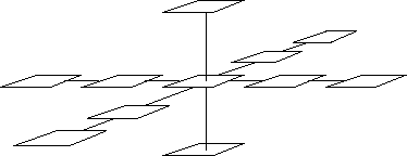
Figure 2.22: The finite difference stencils used in the atmosphere
model. This figure shows for a single grid point both the nine-point
stencil used to simulate horizontal motion and the three-point stencil
used to simulate vertical motion.
The finite difference computations are concerned with the movement, or
fluid dynamics, of the atmosphere. In addition to these dynamics
calculations, the atmosphere model includes algorithms used to
simulate processes such as radiation, convection, and precipitation.
These calculations are collectively termed physics
and use
a range of numerical methods of varying complexity. Data dependencies
within physics computations are restricted to within vertical columns.
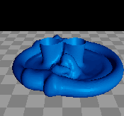
Plate 4
illustrates one of the many phenomena that can be simulated using an
atmospheric circulation model. This shows a potential temperature
isosurface of two thunderstorm downdrafts that hit the ground as
microbursts, then spread out and collide. The surfaces outline the
boundaries of the cold downdrafted air. The collision region contains
wind fields that are dangerous to landing aircraft. The grey tiles
are 1-kilometer squares and the model domain is  km with 50 m resolution.
(GIF 30443 bytes; TIFF 723412 bytes.)
Plate 4: Potential temperature isosurface of two colliding
thunderstorm microbursts. Image courtesy of J. Anderson.
In summary, the atmosphere modeling example is primarily concerned
with performing finite difference computations on a regular
three-dimensional grid. In this respect, it is representative of a
large class of scientific (numeric) computations. The simple, regular
structure of the finite difference method makes it a useful
pedagogical tool, and we shall use it repeatedly in the following
chapters to illustrate issues in algorithm design and performance
analysis.
We now develop parallel algorithms for the atmosphere modeling
problem, proceeding in the stepwise fashion presented in earlier
sections.
The grid used to represent state in the atmosphere model is a natural
candidate for domain decomposition. Decompositions in the x
,
y
, and/or z
dimensions are possible (Figure 2.2).
Pursuant to our strategy of exposing the maximum concurrency possible, we
initially favor the most aggressive decomposition possible, which in
this case defines a task for each grid point. This task maintains as
its state the various values associated with its grid point and is
responsible for the computation required to update that state at each
time step. Hence, we have a total of  tasks, each with
  data and computation per time
step.
The design checklist of Section 2.2.3 does not suggest any
obvious deficiencies in our partition design, so we proceed to
consider communication requirements. We identify three distinct
communications:
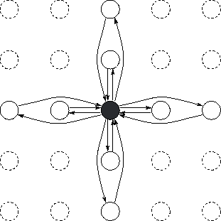
Figure 2.23: Task and channel structure for a two-dimensional finite
difference computation with nine-point stencil, assuming one grid
point per processor. Only the channels used by the shaded task are
shown.
-
Finite difference stencils. If we assume a fine-grained
decomposition in which each task encapsulates a single grid point, the
nine-point stencil used in the horizontal dimension requires that each
task obtain values from eight neighboring tasks. The corresponding
channel structure is illustrated in Figure 2.23.
Similarly, the three-point stencil used in the vertical dimension
requires that each task obtain values from two neighbors.
-
Global operations. The atmosphere model computes periodically
the total mass of the atmosphere, in order to verify that the simulation is
proceeding correctly. This quantity is defined as follows:

where  denotes the mass at grid point (i,j,k)
. This sum
can be computed using one of the parallel summation algorithms
presented in Section 2.4.1.
-
Physics computations. If each task encapsulates a single grid
point, then the physics component of the atmosphere model requires
considerable communication. For example, the total clear sky (TCS) at
level
 is defined as

where level 0 is the top of the atmosphere and cld is the cloud
fraction at level i
. This prefix product
operation
can be performed in
  steps using a variant of the hypercube
algorithm of Section 2.4.1. In total, the physics component
of the model requires on the order of 30 communications per grid point
and per time step.
Let us evaluate this design by using the checklist of
Section 2.3.5. The communication associated with the
finite difference stencil is distributed and hence can proceed
concurrently. So is the communication required for the global
communication operation, thanks to the distributed algorithm developed
in Section 2.4.1. (We might also consider performing this
global operation less frequently, since its value is intended only for
diagnostic purposes.) The one component of our algorithm's
communication structure that is problematic is the physics. However,
we shall see that the need for this communication can be avoided by
agglomeration.
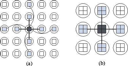
Figure 2.24: Using agglomeration to reduce communication requirements
in the atmosphere model. In (a), each task handles a single point
and hence must obtain data from eight other tasks in order to implement the
nine-point stencil. In (b), granularity is increased to  points, meaning that only 4 communications are required per
task.
Our fine-grained domain decomposition of the atmosphere model has
created  tasks: between
  and
and  ,
depending on problem size. This is likely to be many more than we
require and some degree of agglomeration can be considered. We
identify three reasons for pursuing agglomeration:
-
As illustrated in Figure 2.24, a small amount of agglomeration
(from one to four grid points per task) can reduce the communication
requirements associated with the nine-point stencil from eight to four
messages per task per time step.
-
Communication requirements in the horizontal dimension are relatively
small: a total of four messages containing eight data values. In
contrast, the vertical dimension requires communication not only for
the finite difference stencil (2 messages, 2 data values) but also for
various ``physics'' computations (30 messages). These communications
can be avoided by agglomerating tasks within each vertical column.
-
Agglomeration in the vertical is also desirable from a software
engineering point of view. Horizontal dependencies are restricted to
the dynamics component of the model; the physics component operates
within individual columns only. Hence, a two-dimensional horizontal
decomposition would allow existing sequential physics code to be
reused in a parallel program without modification.
This analysis makes it appear sensible to refine our parallel
algorithm to utilize a two-dimensional horizontal decomposition of the
model grid in which each task encapsulates at least four grid points.
Communication requirements are then reduced to those associated with
the nine-point stencil and the summation operation. Notice that this
algorithm can create at most  tasks: between
  and
and  , depending on problem size. This number is likely to be enough
for most practical purposes.
In the absence of load imbalances, the simple mapping strategy
illustrated in Figure 2.16 can be used. It is clear from
the figure that in this case, further agglomeration can be performed;
in the limit, each processor can be assigned a single task responsible
for many columns, thereby yielding an SPMD program.
This mapping strategy is efficient if each grid column task performs
the same amount of computation at each time step. This assumption is
valid for many finite difference problems but turns out to be invalid
for some atmosphere models. The reason is that the cost of
physics computations can vary significantly depending on model
state variables. For example, radiation calculations are not
performed at night, and clouds are formed only when humidity exceeds a
certain threshold. The sort of variation in computational load that
can result is illustrated in
Plate 5.
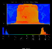
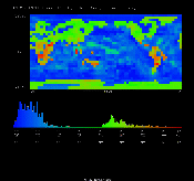
(GIF 28536 and 156403 bytes; RGB 116173 and 919250 bytes.) Plate 5: Load distribution
in an atmosphere model with a 64X128 grid. The figure shows per-point
computational load at a single time step, with the histogram giving
relative frequency of different load values. The left-hand image
shows a time step in which radiation time steps are performed, and the
right-hand image an ordinary time step. Diurnal, land/ocean, and
local variations are visible. Images courtesy of J. Michalakes.
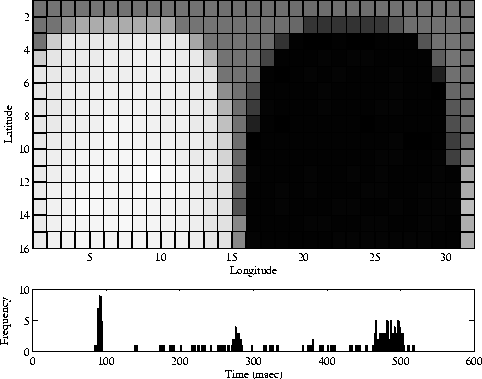
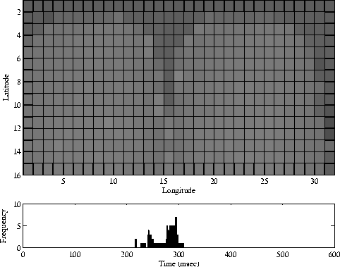
Figure 2.25: Load distribution in the physics component of an atmosphere
model in the absence of load balancing. In the top part of the
figure, shading is used to indicate computational load in each of
 processors. A strong spatial variation is evident. This
effect is due to the night/day cycle (radiation calculations are
performed only in sunlight); hence, there is a temporal variation
also. The bottom part of the figure is a histogram showing the
distribution of computation times, which vary by a factor of 5. These
results were obtained by using a parallel version of the National
Center for Atmospheric Research (NCAR) Community Climate Model (CCM2)
on the 512-processor Intel DELTA computer.

Figure 2.26: Load distribution in the physics component of CCM2
when using a cyclic mapping. A comparison with Figure 2.25 shows that
load imbalances are reduced significantly.
Empirical studies suggest that these load imbalances can reduce
computational efficiency by 20 percent or more
(Figure 2.25; see also
Plate 5).
In many circumstances, this performance loss may be regarded as
acceptable. However, if a model is to be used extensively, it is
worthwhile to spend time improving efficiency. One approach is to use
a form of cyclic mapping: for example, allocating each processor tasks
from western and eastern and from northern and southern hemispheres.
Figure 2.26 shows the reduction in load imbalance that can
be achieved with this technique; this reduction must be weighed
against the resulting increase in communication costs.
The design of a parallel atmosphere model has proved to be
straightforward process, in that most design choices are clear-cut. A
two-dimensional domain decomposition of the model grid results in a
need for both local communication between tasks handling neighboring
grid points and a parallel summation operation.
One unanswered question concerns whether load-balancing algorithms
should be incorporated into the model. Because load balancing adds to the
complexity of the overall design, this decision requires both
performance data (of the sort presented in Figure 2.25) and
information about the expected use of the parallel model. Another
question, addressed in Chapter 4, is how the
atmosphere model will fit into a larger framework such as the climate
model of Figure 2.3.
![[DBPP]](pictures//asm_color_tiny.gif)


![[Search]](pictures//search_motif.gif)
Next: 2.7 Case Study: Floorplan Optimization
Up: 2 Designing Parallel Algorithms
Previous: 2.5 Mapping
© Copyright 1995 by Ian Foster

 and
and  are latitude and longitude,
z
is height, u
and v
are horizontal components of
velocity, p
is pressure,
  is density, T
is
temperature, f
is Coriolis force, g
is gravity,
F
and Q
are external forcing terms,
  is specific
heat, and a
is the earth's radius.
![[DBPP]](pictures//asm_color_tiny.gif)


![[Search]](pictures//search_motif.gif)
 , with
  in the range 15--30,
  , and
, and  in the range 50--500
(Figure
  is viewed as
being adjacent to
  and
and  .
A vector of values is maintained at each grid point,
representing quantities such
as pressure, temperature, wind velocity, and humidity.


 km with 50 m resolution.

 tasks, each with
  data and computation per time
step.


 denotes the mass at grid point (i,j,k)
. This sum
can be computed using one of the parallel summation algorithms
presented in Section
  is defined as

 is the cloud
fraction at level i
. This prefix product
operation
 steps using a variant of the hypercube
algorithm of Section
 points, meaning that only 4 communications are required per
task.
 tasks: between
  and
and  ,
depending on problem size. This is likely to be many more than we
require and some degree of agglomeration can be considered. We
identify three reasons for pursuing agglomeration:
 tasks: between
  and
and  , depending on problem size. This number is likely to be enough
for most practical purposes.


 processors. A strong spatial variation is evident. This
effect is due to the night/day cycle (radiation calculations are
performed only in sunlight); hence, there is a temporal variation
also. The bottom part of the figure is a histogram showing the
distribution of computation times, which vary by a factor of 5. These
results were obtained by using a parallel version of the National
Center for Atmospheric Research (NCAR) Community Climate Model (CCM2)
on the 512-processor Intel DELTA computer.