3.5 Experimental Studies

  Discussion in preceding sections has emphasized analytic modeling of performance. Yet parallel programming is first and foremost an experimental discipline. The flexibility and ease of modification of software on the one hand, and the complexity of parallel computer systems on the other, mean that approaches to parallel program design based entirely on theory are rarely cost effective. The role of modeling is most often to assist in what is essentially an experimental process, by guiding experiment and explaining results.

Experimental studies can be used in early design stages to determine values for parameters used in performance models, such as computation time per grid point, average depth of a search tree, message startup cost, and message transfer costs. They can also be used after programming begins, to compare observed and modeled performance.

Next we review several sometimes subtle issues that can arise during experimental studies.

3.5.1 Experimental Design

  The first step in an experimental study is to identify the data that we wish to obtain. For example, when calibrating a performance model we may be interested in determining the execution time of a sequential version of our application as a function of problem size in order to determine . Or, we may need to measure the execution time of a simple message-passing testbed program in order to determine and .

Normally, experiments are performed for a range of data points---different problem sizes and/or processor counts. By maximizing the number of data points obtained, we reduce the impact of errors in individual measurements. When empirical data are used to evaluate the quality of an implementation, a range of data points also allows us to estimate the accuracy of the model and to identify regimes in which it is inadequate.

The next step in an experimental study is to design the   experiments that will be used to obtain the required data. The critical issue here is to ensure that our experiments measure what we intend to measure. For example, if a program comprises an initialization step followed by a long series of iterations, and our performance model deals only with the cost of an iteration, then that is what we need to measure.

3.5.2 Obtaining and Validating Experimental Data

The principal challenge when performing experiments is to obtain accurate and reproducible results. Execution times can be obtained in various ways; which is best will depend on both our requirements and the facilities available on the target computer. A straightforward but potentially time-consuming approach is to incorporate code into our program that calls system timer routines to determine elapsed time. In principle, we should make these calls on every processor and then take the maximum time. However, we can often identify a reference processor that does not start or finish appreciably later or sooner than others, and measure times on this processor alone. Alternatively, we can use a profiling or tracing tool that obtains timing data automatically. We discuss specific tools in Chapter 9.

Experiments should always be repeated to verify that results are reproducible. Generally, results should not vary by more than a small amount---2 or 3 percent is a lot if one is trying to fine-tune algorithms. Possible causes of variation include the following.

•   A nondeterministic algorithm. Programs may use random numbers   or may explore a search space or allocate work to processors in a time-dependent manner (as in the search algorithm of Section 2.7). Nondeterminism due to random numbers can be controlled by using a reproducible parallel generator (Chapter 10). Nondeterminism due to time-dependent execution is more problematic. One solution is to perform a large number of trials. Another is to normalize execution times by dividing them by some measure of the amount of work done, such as search tree nodes visited.

• An inaccurate timer. The timer used to obtain execution times may have limited resolution or be inaccurate. If resolution is limited, we can improve accuracy by increasing execution time, for example by performing more iterations or by solving the same problem several times. If the timer is inaccurate, we need to find another way to determine execution times.

• Startup and shutdown costs. The time required for system management functions concerned with the acquisition of processors, loading of code, allocation of virtual memory, deallocation of processors, etc., can vary significantly according to the state of the system. Timings are often more accurate if these system-dependent components are excluded. Hence, we may start a timer after a program is loaded and stop it once a solution has been computed.

• Interference from other programs. On a nondedicated machine, other users may compete for shared resources such as processors, network bandwidth, and I/O bandwidth. Timings may also be perturbed by system functions such as accounting and backups that execute occasionally. Note that competition can occur even when processors are dedicated to our application. For example, a computer in which processors are connected in a 2-D mesh (Section 3.7.2) may be partitioned into disjoint submeshs. Yet I/O requests generated by programs executing in one submesh may need to traverse our submesh to reach I/O devices, thereby consuming bandwidth.

• Contention. On some computers, the time required for a communication operation can increase when several processors communicate at the same time. For example, an Ethernet-connected LAN can carry only one message at a time, and senders must back off and resend when messages collide. An unfortunate schedule can result in repeated resendings, thereby increasing execution time. In Section 3.7, we describe advanced modeling techniques that can account for some such effects.

• Random resource allocation. The operating system may use a random processor allocation strategy, which will affect execution times if communication costs depend on processor location in a network (see Section 3.7). If possible, the same allocation should be used for all experiments.

Studies of variability in experimental results can help us to identify sources of error or uncertainty in our measurements. However, even when results are reproducible, we still have no assurance that they are correct. Confidence in our results can be increased by measuring the same thing several different ways and verifying that the results of these redundant measurements are consistent. For example, in addition to measuring the time taken in individual program components, we can measure the total time for the entire program.

3.5.3 Fitting Data to Models

  When experimental studies are performed for calibration purposes, we   fit results to the function of interest to obtain values for unknown parameters. A fit can be performed graphically by plotting data points and estimating the fit. For example, if the function is

we can plot the data points as a function of L and draw a straight line that fits these points. The slope of this line will be , and the intercept of the axis when L=0 will be .

  Alternatively, and more accurately, we can perform a least-squares fit of the function with the data. (Mathematical packages such as Mathematica and Matlab incorporate fitting functions.) A least-squares fit involves a minimization of the sum of the squares of the differences between the observations, obs (i) , and the corresponding function values, f (i) :

For example, when fitting the function with observations of T for different values of N in order to determine the value , we minimize

When fitting to execution times for different numbers of processors, the method just described gives less weight to the (presumably smaller) times on larger numbers of processors. Yet these are typically the times of greatest interest. Hence, we can use a scaled least-squares fit in which the difference between observation and function value is scaled by the observation, as follows:

Example . Determining Computation Time ()

We consider the problem of determining the computation cost per grid   point in the finite difference problem. Recall that we have modeled this cost as follows (Equation 3.2):

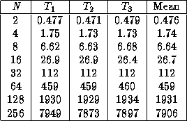
In this equation, is the parameter that we wish to determine, and N is a value that we can vary while measuring performance. (For simplicity, we keep Z fixed.) Table 3.2 gives execution times measured on a Sun SPARC 2 workstation. Experiments were performed when the machine was idle but not in single-user mode; hence, there might have been a small amount of background activity. Each experiment was repeated three times so that we could study variability; the table also lists the means of each set of three values. The repeated experiments show little variation in total execution time.

 
Table 3.2: Execution times in milliseconds for a single time step of the finite difference code on a Sun SPARC 2, with Z=10 .  

 
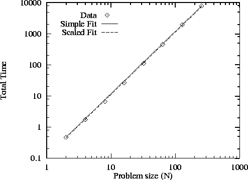
Figure 3.9: Simple and scaled least-squares fits of the function to finite difference execution times on a Sun SPARC 2 workstation. Notice the use of logarithmic scales. 

 
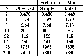
Table 3.3: Execution times predicted for finite difference code on Sun SPARC 2, with Z=10 (milliseconds).  

Figure 3.9 shows simple and scaled least-squares fits of Equation 3.2 to the data in Table 3.2. The two fits correspond to values of 0.0120 msec and 0.0112 msec, respectively. The execution times predicted by the two models are     shown in Table 3.3. As expected, the simple fit is more accurate for larger N , while the scaled fit is better for smaller N ; both are good enough for most practical purposes. These results suggest that the hypothesized performance model, , is an adequate characterization of finite difference computation time.